Mech-DLK 3.0.1 Training Parameter Tuning and Model Optimization Guide

Alina · October 16, 2026, 6:23am

Mech-DLK 3.0.1 Training Parameter Tuning and Model Optimization Guide

When model performance is unsatisfactory, first check whether the input images are clear and whether the data covers on-site variations, and then adjust the training parameters. Simply increasing parameter values usually lengthens training time and increases GPU memory usage, but does not address the root causes of missed or false detections.

This guide is intended for all Mech-DLK users and requires no prior knowledge of deep learning algorithms. It focuses on the following information:

Which Mech-DLK tools to use and how to set the training parameters for different symptoms;
Why these adjustments may improve model performance;
How to balance model accuracy, training time, inference time, and GPU memory usage.

This guide does not cover derivations of algorithmic principles, troubleshooting of uncommon issues, or the complete steps of image acquisition and labeling; for these operations, refer to the official manual links provided in this document.

How to use this guide: Jump to the corresponding section from the table below based on the symptom you encounter. Change only one main factor in each experiment, and compare results using the same validation set. For allowed parameter ranges and common default values, see the Appendix: Mech-DLK 3.0.1 Key Parameters Quick Reference.

Quick Lookup by Symptom

Symptom	Related section
Unsure what to check before your first training run	Checks Before Parameter Tuning
False detections caused by fixed backgrounds, fixtures, reflections, or irrelevant text	Image Input and Labeling Tools
Recognition fails only under specific brightness, angle, or position conditions	Data Augmentation
Unsure how to set parameters such as Model type, Batch size, and Epochs	Training Parameters
Tiny defects or small targets are missed in large images	Input Image Size: Input Size and Small Targets
Need to reduce GPU memory usage or improve training efficiency	Balancing GPU Memory and Resources
Insufficient GPU memory reported during training	Procedure for Handling Insufficient GPU Memory
The model fails on only a few samples in a new batch	Model Finetuning
One project needs to handle multiple tasks such as positioning, classification, defect detection, or character recognition	Using Serial and Parallel Modules

1. Checks Before Parameter Tuning

Before tuning parameters, check the following items in order and locate the problem starting from the most visible symptom. The earlier an item appears, the higher its priority.

Check the original images: Check whether small targets, defects, or character features are clear in the original images, and whether there are out-of-focus areas, overexposure, underexposure, or strong reflections. If the images are not clear, adjust the light source, exposure, focal length, or camera mounting first before making any further adjustments.
Check the Zoom Preview window: If the original images are clear, open the Zoom Preview window to confirm that targets or defects remain clear at the current input size. If targets are no longer clearly visible after scaling, use an ROI (region of interest), grid cutting, or increase the Input image size.
Check labeling and samples: Check whether there are missing labels, incorrect labels, or inconsistent boundary criteria, and whether each type of on-site variation has corresponding samples. If labeling problems exist, correct the labels first and add representative OK/NG images.
Check whether the data covers on-site variations: Check whether recognition fails only under specific brightness, angle, position, or batch conditions. If so, prioritize adding real samples captured under those conditions, and then configure data augmentation to match the on-site variations.
Check training results: Check whether performance on the training set and the validation set is consistent. If the model performs well on the training set but poorly on the validation set, check for overfitting and data distribution issues; if accuracy is still improving when training ends, increase the number of epochs appropriately.
Check task boundaries: Check whether a single module handles positioning, classification, and defect detection at the same time, making failure cases difficult to analyze. If so, split the tasks using serial or parallel module combinations; after the split, each module learns only well-defined targets.

2. Image Input and Labeling Tools

The ROI, image preprocessing, masks, and grid cutting determine which image information the model receives, and they should usually be configured before training parameters are adjusted. For detailed instructions on using each tool, see the official labeling tool instructions.

1. ROI: Removing Irrelevant Backgrounds

Applicable symptom: The detection region is roughly at the same position across images, and the target occupies only a small part of the original image.
Effect: Removes irrelevant backgrounds, reduces interference, and makes the target occupy a larger proportion of the input image.
Usage tips: When setting the ROI, ensure it covers the target objects in all images, accounting for variations in their positions and including any surrounding context needed for inspection. Avoid drawing the ROI too tightly around the target objects.
Limitations: A fixed ROI is not suitable when target object positions or angles vary significantly. You can first use a Fast Positioning or Object Detection module to correct positions, and then use the cropped images as input to downstream modules. If the target must be inspected based on surrounding structures, excessive cropping may remove the context required for inspection.

2. Image Preprocessing: Correcting Issues Common to All Images

Image preprocessing is applied consistently to all images in the project and is suitable for correcting common imaging issues, whereas data augmentation is applied randomly during training only. The two cannot replace each other. For the parameter definitions, see the official parameter descriptions.

Tool	Applicable symptom	Adjustment direction	Notes
Brightness	All images are uniformly too dark or too bright	Increase moderately when too dark; decrease moderately when too bright	Excessive adjustment causes highlight saturation, loss of details in dark areas, or amplified noise
Contrast	Insufficient contrast between target edges or textures and the background	Increase moderately to make the differences more distinct; decrease if texture details or noise become overemphasized	If detecting subtle defects depends on small grayscale differences, compare failure cases in the validation set before and after the adjustment
Illumination normalization	Overall lighting varies across times or batches	Enable when the judgment does not depend on absolute brightness	If brightness itself is the basis for the OK/NG judgment, do not over-normalize
Adaptive color balancer	Images generally have a color cast or are over- or undersaturated	Use to correct color casts and make color rendering more consistent across images	If color is a class or defect feature, preserve actual color differences

Training, validation, and deployed inference must use the same preprocessing workflow. Otherwise, differences between the images used for training and those used for on-site inference may degrade model performance.

3. Masks: Excluding Fixed Interference Areas

Applicable symptom: Fixed fixtures, standard weld spots, irrelevant text, borders, or reflective areas frequently cause false detections.
Effect: Areas covered by masks are not involved in model training.
Usage tips: A single image mask applies only to the current image and is suitable when interference areas are not in fixed positions. A single image mask can be copied or batch-pasted to similar images. A global mask applies to all images and is suitable only when target object positions are consistent and the interference areas are fixed.
Limitations: Masks should completely cover the interference areas, but must not cover real targets, defects, or the surrounding context required for judgment. When target object positions vary significantly, first correct positions with a Fast Positioning or Object Detection module, and then use a global mask.

4. Grid Cutting: Preserving Tiny Features in Large Images

Applicable symptom: Defects are no longer clearly visible after the entire image is scaled down, and they may be distributed across a large area of the image.
Effect: Splits large images into multiple cell images, so that tiny defects and text features occupy more pixels in the input images.
Procedure:
1. Complete labeling on the original image first, and then set the number of rows and columns.
2. Start with a small number of rows and columns; in the Zoom Preview window, confirm that defects are clear and complete within the cell images.
3. If a labeled area crosses a grid boundary, set Edge Expansion to prevent grid cutting from splitting the defect across multiple cell images and affecting the final segmentation result.
4. Use the Grid Selection Tool to select the cell images that contain defects, along with an appropriate number of representative OK cell images.
Limitations and costs: Increasing the number of rows and columns reduces GPU memory usage per cell image. However, it also produces more cell images, which increases the overall training time and end-to-end inference time. Use the fewest grid cells needed to keep the defects clearly visible.

For a complete walkthrough, see the official tutorial Detecting Small Defects in Large Images.

3. Data Augmentation

Data augmentation is used to simulate on-site variations that are not sufficiently covered by the current data. After an augmentation option is selected, the augmentation occurs with a certain probability only during training, and a value is randomly selected from the specified range. If an augmentation may compromise key features, adjust its range to reduce its effect or disable it. For the definitions and default ranges of each parameter, see the official parameter descriptions.

Parameter	Simulated real-world variation	When to enable	When to reduce or disable
Brightness	Changes in lighting intensity, lamp aging, exposure changes	Reasonable brightness fluctuations exist across different times of day or devices	Detecting subtle defects depends on small grayscale differences; overexposure or underexposure occurs after augmentation
Contrast	Differences in light–dark contrast and material reflectivity	Material or lighting causes the target contrast to vary	Textures are flattened, or noise is noticeably amplified
Translation	Position changes of target objects, bins, or pallets	Target object positions vary in the field of view	The station is fixed, or positional correction has already been performed.
Rotation	Target object pose changes	Target object orientations are random, and orientation does not affect class or judgment	Character orientation, front/back sides, or assembly orientation carry business meaning
Scale	Changes in camera-to-object distance, object size, or height	The distance between the target object and the camera actually varies	Small targets or small defects may disappear when scaled down
Flip horizontally / Flip vertically	Mirrored variations	The semantic meaning of the image remains unchanged after flipping	Text, left–right parts, top–bottom orientations, or asymmetric structures

For small-target scenarios, check the scale augmentation first: if key features disappear in the Zoom Preview window after scaling down, set the lower limit of Scale to 0% and keep only the augmentation range that does not distort the features. The default augmentation ranges are conservative. For example, Brightness and Contrast default to -10%–10%, while Rotation and Scale are disabled by default. Before widening a range, confirm that the corresponding variation genuinely exists on site.

4. Training Parameters

Determine the training parameters in the following order: Model type → Input image size → Batch size → Epochs → Eval. interval → GPU ID and Max num of training objects. Do not tune a later parameter until the preceding parameters have been determined. For example, confirm that defects remain visible at the current Input image size before adjusting Batch size. For the interface location and default values of each parameter, see the official training parameter descriptions and Train a Model.

1. Model Type: Choosing by Task Characteristics

The Defect Segmentation and Text Detection modules provide the High-accuracy and High-speed model types. For the first training, you can use the High-speed model to quickly verify whether the images and labels are reasonable with lower resource usage; if small defects or weak features are poorly recognized, test the High-accuracy model.
The Instance Segmentation module provides the Integrated model and the Tightly packed long object model. Use the Integrated model in most cases; when target objects are densely arranged, closely attached, or elongated, test the Tightly packed long object model first.

The High-accuracy model usually requires more GPU memory and longer training and inference times. Changing the model type is likely to improve performance only after the images, labels, and input image size have been properly configured.

Verification: Use the same validation set to compare the missed detections, false detections, training time, and inference time of the two models.

2. Input Image Size: Input Size and Small Targets

Input image size specifies the width and height, in pixels, of the images used as network input for training and inference. The principle for selecting it is not “the larger the better,” but the smallest size that still preserves the smallest key features. After grid cutting is enabled, this parameter refers to the size of the cell images used as network input.

When images are scaled proportionally, use the following formula to estimate the feature size after scaling:

Feature pixels after scaling ≈ feature pixels in the original image × Input image size ÷ image side length before processing

For example, if the original image is 4000 pixels wide and a defect is about 10 pixels wide, scaling the original image down to a width of 512 pixels leaves the defect only 1.3 pixels wide, which is usually too small for stable recognition. If you first crop a valid region 500 pixels wide and then scale it to 512, the defect remains about 10 pixels wide.

Increase: Retains more details and may reduce missed detections of small targets; peak GPU memory increases significantly, and training and inference take longer.
Decrease: Reduces peak GPU memory and training time; small targets may become unrecognizable due to scaling.
How to set: Use the Zoom Preview window to select the smallest size at which the smallest key features remain visible; the model must be retrained after this parameter is changed.
Verification: Compare missed and false detections on a fixed validation set, and check the peak GPU memory in the Training center.

If key features are unclear in the Zoom Preview window, follow the sequence below. After each adjustment in the flowchart, compare missed detections, false detections, and resource usage on a fixed validation set.

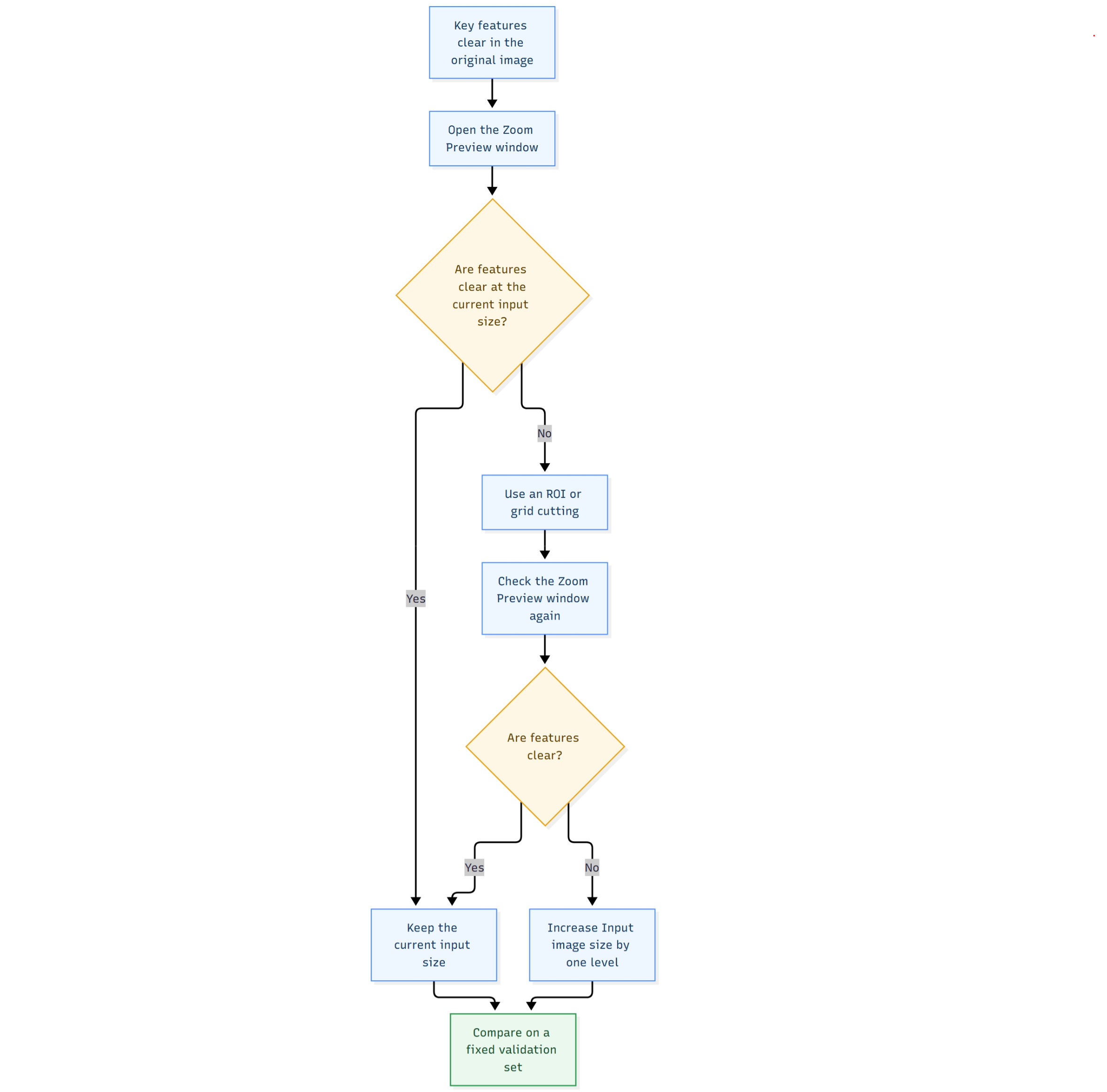
The input size increases both the width and height of the image, so resource consumption grows mainly with area. Taking 512×512 pixels as the baseline: when the side length increases to 1024, the area becomes (1024 ÷ 512)² = 4 times larger; when it increases to 2048, the area becomes 16 times larger. Actual GPU memory growth is affected by the algorithm module and the software implementation, and may not exactly match the area ratio, but Input image size is usually the parameter with the most noticeable impact on GPU memory and speed.

3. Batch Size: Number of Images Trained at One Time

Batch size is the number of images processed by the GPU in a single training step. For example, when Batch size is 2, two images are grouped into one batch and processed together in a single training step.

Increase: Peak GPU memory increases; when GPU memory is sufficient, training efficiency improves and total training time is shortened.
Decrease: Peak GPU memory decreases; the total time required to complete the same amount of training usually becomes longer.
How to set: Determine the Model type and Input image size first, and then increase Batch size step by step from the default value; decrease it step by step when GPU memory becomes insufficient. Do not reduce the input size to a level where key features are no longer visible just for a larger Batch size.
Verification: Observe the changes in peak GPU memory and training time in the Training center.

4. Epochs: Number of Complete Passes Through the Training Set

Epochs is the total number of times the model completely passes through the training set.

Increase: Total training time increases. If training has not converged and the number of failure cases in the validation set continues to decrease, increasing Epochs may further improve performance; if the value is too high, the model may overfit the training set, and performance on the validation set and on site may instead deteriorate.
Decrease: Total training time decreases. Insufficient training may lead to underfitting and missed detections.
How to set: Use the software default value for the first training; increase it appropriately for tasks with high recognition difficulty or strict accuracy requirements. Increase it gradually only when the loss and the number of failure cases in the validation set are still decreasing at the end of training; if model performance on the training set improves while performance on the validation set deteriorates, reduce Epochs and check the data coverage and augmentation ranges.
Verification: Observe the accuracy and loss curves in the training charts, and the change in the number of failure cases in a fixed validation set.

In Mech-DLK 3.0.1, the allowed range of Epochs is 1–10000. 10000 is the allowed upper limit, not the default or recommended value. The larger the dataset, the more training steps each epoch contains, so do not mechanically increase Epochs just because the dataset is large.

5. Eval. Interval: Model Evaluation Interval

Eval. interval is the number of epochs between two model evaluations, with a default value of 10.

Increase: The number of evaluations decreases and training is faster; however, with fewer opportunities to record the best-performing model, a temporary peak in model performance may be missed.
Decrease: Evaluations become more frequent, making it easier to select the optimal model; the evaluation overhead increases and training slows down.
How to set: Keep the default value for the first training. Decrease it for small datasets or when training curves fluctuate noticeably; increase it moderately for long training runs with stable curves.
Verification: Compare the total training time and the performance of the optimal model on a fixed validation set.

6. GPU ID and Max Num of Training Objects

GPU ID: On multi-GPU devices, you can specify the GPU used by the training task, and view the GPU memory usage and task queue of that GPU in the Training center. Selecting a GPU ID does not mean that a single training task will automatically use multiple GPUs.
Max num of training objects: Visible in the Object Detection and Instance Segmentation modules. It limits the maximum number of targets per image that participate in training, and it is disabled by default. Set it slightly higher than the actual maximum number of targets in a single on-site image: setting it too small causes targets to be dropped; when set appropriately, it usually reduces wasted computation and speeds up inference on some images.

5. Balancing GPU Memory and Resources

The goal of parameter tuning is not simply to reduce GPU memory usage, but to choose an appropriate combination of model performance, training time, inference time, and GPU memory usage.

Peak GPU memory determines whether training can start and continue. It is the maximum amount of GPU memory used during training. If it exceeds the available GPU memory, training may fail to start or may stop unexpectedly. Use the GPU memory usage displayed in the Training center as the definitive reference.

Peak GPU memory can be approximated as:

Fixed model overhead + Batch size × intermediate feature overhead per image + additional overhead such as the number of targets

This relationship is only for understanding trends. Actual usage also depends on the algorithm module, model type, GPU, and driver.

1. Impact of Each Parameter on Resources

Parameter or tool	Impact on peak GPU memory	Impact on training or inference time	Setting principle
Input image size	High; increasing the side length increases both width and height	Usually noticeably slower	Ensure key features are clear first, and then choose the smallest usable value
Batch size	Relatively large; the more images processed at once, the higher the usage usually	Can improve training efficiency within the GPU memory limit	Increase step by step after the input size is determined
High-accuracy model / High-speed model	The High-accuracy model usually uses more GPU memory	The High-accuracy model usually requires longer training and inference times	Use the high-speed model for the first training, and then verify whether the high-accuracy model is necessary
Max num of training objects	More targets lead to higher additional overhead in some modules	May increase processing time	Slightly higher than the actual on-site maximum
ROI or positioning-based cropping	Indirectly reduces the input overhead of downstream modules	Usually beneficial to downstream efficiency	Remove irrelevant areas first
Grid cutting	Reduces GPU memory usage per cell image	The number of cell images increases, and the overall time may become longer	Use the minimum number of splits
Epochs	Little to no effect on per-step peak GPU memory	Mainly increases total training time	Increase only when training has not converged
Eval. interval	Little to no effect on peak GPU memory during training	The larger the interval, the lower the evaluation overhead	Used to balance evaluation frequency and training time

2. Combining Input image size and Batch size

Use the Zoom Preview window to determine the Input image size that preserves the smallest key features.
Start training with the default Batch size of the module, and observe the peak GPU memory in the Training center.
When GPU memory headroom is sufficient, increase Batch size step by step, and observe the peak GPU memory and training time again.
When insufficient GPU memory is reported, decrease Batch size step by step.
If training still fails after Batch size is reduced to 1, use an ROI, positioning-based cropping, or grid cutting to reorganize the input; if the issue persists, further reduce the Input image size or switch to a high-speed model.

For detection performance, ensuring that key features are clearly visible usually takes priority over a larger Batch size.

3. Procedure for Handling Insufficient GPU Memory

An insufficient GPU memory message during training means that the current peak GPU memory exceeds the available GPU memory, which causes training to fail to start or be interrupted. Follow the sequence below, and after each step is completed, retrain and check the GPU memory usage:

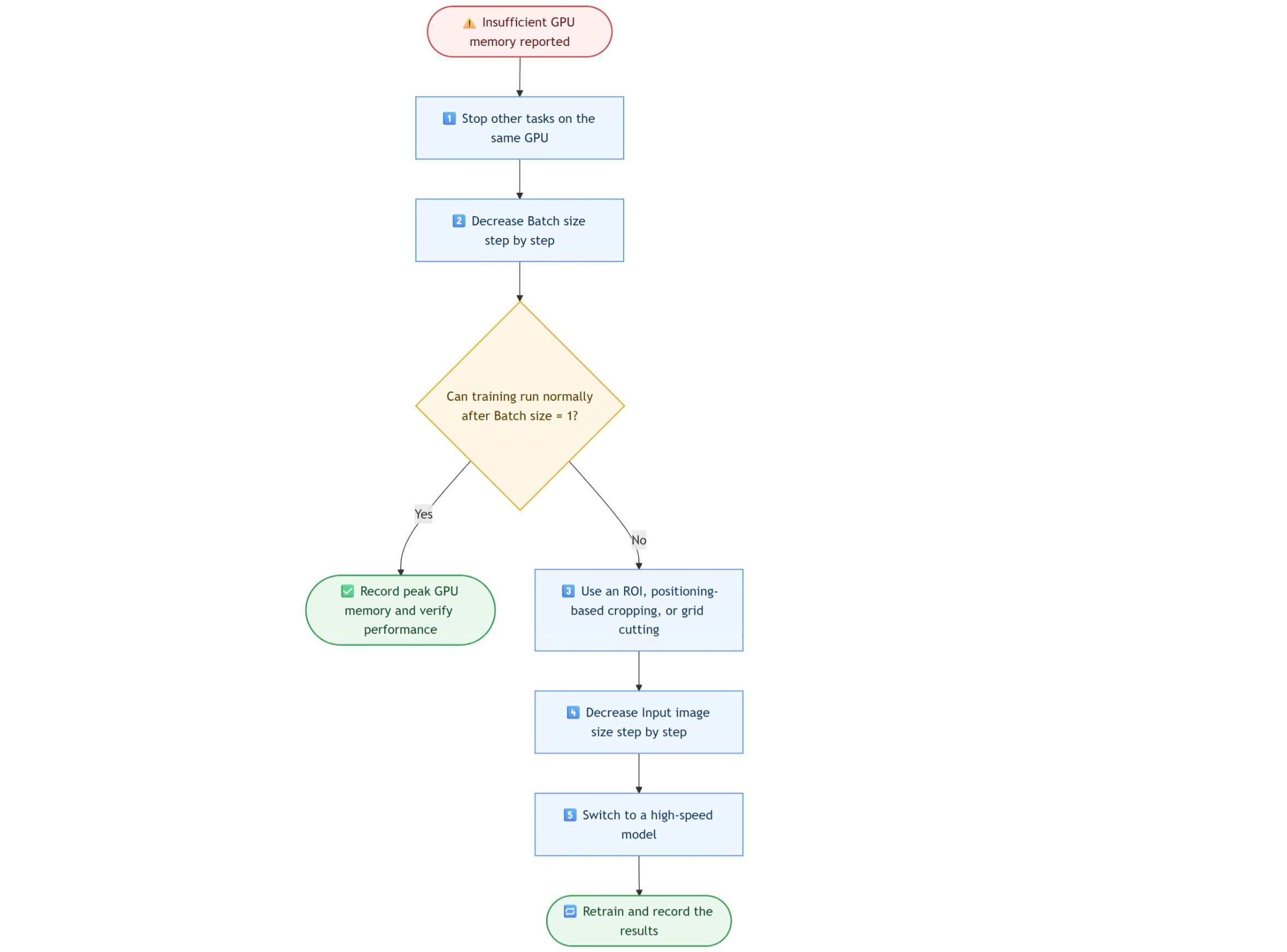
Training, validation, and smart labeling tasks, as well as other GPU programs, can all occupy GPU memory. Avoid configurations whose peak GPU memory is close to the GPU limit. Leaving some headroom helps prevent intermittent failures.

4. Choosing Between High Resolution and Grid Cutting

Assume that the full image requires an input size of 4096 for tiny defects to be visible. The alternative is to split the image into a 2×2 grid, producing four cell images, each with an input size of 2048. The two approaches may preserve similar local details, but their resource costs differ:

Approach	Peak GPU memory	Training and inference time	Applicable scenario
Full image + 4096	High usage in a single pass	Fewer processing passes, complete context	Complete context is required, and GPU memory is sufficient
2×2 grid cutting + 2048	Lower usage per cell image	Processes up to 4 cell images, so the overall time may increase	Tiny defects are distributed across the large image, and GPU memory usage per pass must be controlled

If defects appear only in a fixed region, an ROI is usually more efficient than splitting the entire image; if defects may appear anywhere in the large image, grid cutting is usually more controllable than continuously increasing the input size of the full image. Ultimately, compare the detection rate, peak GPU memory, and end-to-end inference time together.

5. Adjustments That Do Not Reduce Peak GPU Memory

Reducing Epochs only shortens the total training time and usually does not reduce the per-step peak GPU memory.
Increasing Eval. interval mainly reduces the number of evaluations and is not the preferred way to resolve insufficient GPU memory.
Model finetuning can reduce the number of training epochs and the data preparation cost, but training still needs to store intermediate features, so peak GPU memory may not decrease noticeably.

6. Model Finetuning

When a deployed model performs poorly only on a few new batches, under certain lighting conditions, or on difficult samples, use model finetuning to update the existing model while maintaining its current performance and reducing training time. For instructions, see the official Iterate a Model page.

Prerequisites:

Model finetuning is available only in Developer mode.
The Fast Positioning, Pick Anything V2, and Object-Bin Segmentation modules do not support model finetuning for now; to improve these models, add more data and retrain them.

The software provides two finetuning methods:

Self finetuning: Continues training based on the current model in the original project; for the Instance Segmentation module, you also need to select Self finetuning in the Model finetuning settings.
Deep learning model finetuning: Adapts an existing .dlkmp model file to the current scenario and can be used to fine-tune general models.

Follow these steps:

Collect images on which the model performs poorly, label them accurately, and add them to the training set.
Keep a portion of representative images from the old scenarios to prevent the model from adapting only to the new failure cases.
In the Training Parameter Settings window, select the Model finetuning tab, and then enable Finetune. Set Epochs to 50–80 as a starting point (the value recommended in the official Iterate a Model instructions), and then adjust based on the validation results.
Use a validation set that covers both new and old scenarios to compare missed detections, false detections, and inference time before and after finetuning.

Note: When the class definitions, imaging method, or task structure has changed significantly, retrain the model instead of attempting model finetuning.

7. Using Serial and Parallel Modules

Mech-DLK supports combining multiple algorithm modules in a tree structure within one project using serial, parallel, or hybrid serial-parallel combinations. Data can be labeled and models can be trained and validated independently for each module. The modules are then exported as a single multi-model package for unified execution and maintenance. For detailed rules, see the official Introduction to Tree-Structured Algorithm Modules.

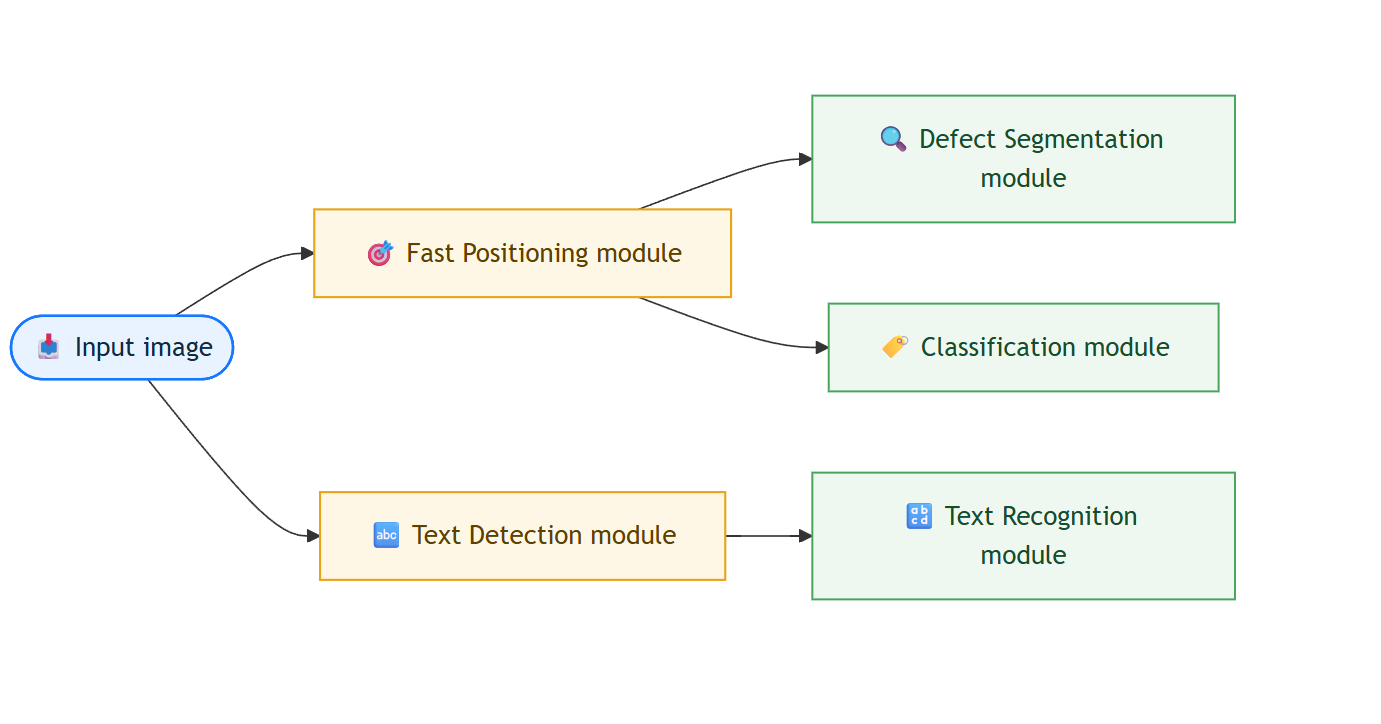
In the figure, “Fast Positioning module → Defect Segmentation module” and “Text Detection module → Text Recognition module” are serial combinations. The Defect Segmentation and Classification modules share the output of the Fast Positioning module, forming parallel branches. The entire workflow is a hybrid serial-parallel combination.

1. Serial Module Mode

In serial module mode, multiple modules are connected in sequence, and the output of one module is used as the input of the next. This combination is suitable for workflows with clear sequential dependencies.

Fast Positioning module → Defect Segmentation module: Normalize positions and orientations first, and then inspect local defects.
Object Detection module → Classification module: Locate each object first, and then determine its type or class.
Text Detection module → Text Recognition module: Find the text regions first, and then recognize the characters.

In a serial structure, targets missed by an upstream module never reach the downstream modules, so prioritize preventing missed detections in the upstream modules. After an upstream model is updated, re-validate the performance of the downstream modules.

2. Parallel Module Mode

In parallel module mode, multiple modules at the same level process the same input independently and produce separate results. This combination is suitable when the same image requires multiple independent analyses, such as classification, defect segmentation, and text detection. Parallel combinations make each module easier to maintain independently, but the total inference time generally increases with each additional branch.

3. Hybrid Serial-Parallel Combination

First use a Fast Positioning module to correct the target object positions, and then run the Defect Segmentation, Classification, and Text Detection modules in parallel. This arrangement is suitable for comprehensive quality inspection tasks. Separating the tasks allows each module to handle only well-defined targets, making failure cases easier to trace. Measure the end-to-end inference time of the complete workflow as well.

4. Combination Restrictions

Only the Text Recognition module can be connected in series under a Text Detection module; no other modules can be connected in series after a Text Recognition module.
The Pick Anything V2 module and the Object-Bin Segmentation module can only be connected in series with the Input module, and cannot be connected in series or in parallel with other modules.

8. Typical Scenarios and Recommended Paths

Typical scenario	Recommended path
Tiny defects in large images	Improve imaging → Zoom Preview → ROI or grid cutting → Input image size → High-accuracy model
Large position variations of small targets	Fast Positioning or Object Detection module → cropped images as input → Classification or Defect Segmentation module
Dense, elongated, or closely attached target objects	Tightly packed long object model → Max num of training objects → Input image size
Failures only under some lighting conditions	Add real samples → Brightness/Contrast data augmentation → check whether preprocessing is too strong
Text orientation issues or character confusion	Text Detection module → orientation correction → Text Recognition module; disable unreasonable rotation and flip augmentation
A few failure cases in a new batch	Label and add the failure-case images → model finetuning → validate on both new and old scenarios
Good training set performance but poor on-site performance	Check data distribution, labeling criteria, preprocessing consistency, data augmentation, and overfitting; do not blindly increase Epochs

9. Experiment Records and Validation

Record at least the following for each training:

Software, project, dataset, classes, and model versions;
ROI, preprocessing, masks, grid cutting, and module structure;
Model type, Input image size, Batch size, Epochs, Eval. interval, GPU ID, and Max num of training objects;
Total training time, peak GPU memory, and end-to-end inference time;
Missed detections, false detections, classification errors, and boundary issues on the fixed validation set;
The single change made this time, the symptom it resolved, and any side effects it introduced.

Model optimization loop: Review failure cases → identify the cause → change one main factor → compare using the same validation set → keep the effective configuration.

Appendix: Mech-DLK 3.0.1 Key Parameters Quick Reference

1. Allowed Parameter Ranges

Parameter	Allowed range or options
Epochs	1–10000
Batch size	1 / 2 / 4 / 8 / 16 / 32 / 64 / 128
Input image size (general)	256 / 512 / 640 / 768 / 1024 / 1536 / 2048 / 2560 / 3072 / 4096
Input image size (Classification module)	112 / 224 / 448 / 640 / 768 / 1024 / 1536 / 2048
Input image size (Unsupervised Segmentation module)	128 / 256 / 512 / 640 / 768 / 1024 / 1536 / 2048
Input image size (Text Recognition module)	N/A
Brightness augmentation	-100%–100%
Contrast augmentation	-100%–100%
Translation augmentation	-50%–50%
Rotation augmentation	-180°–180°
Scale augmentation	-99%–99%
Image preprocessing: Brightness, Contrast	-100%–100%

2. Common Default Values

Parameter	Default value
Batch size	1 for the Fast Positioning module; 2 for the Object Detection, Instance Segmentation, Defect Segmentation, and Text Detection (High-accuracy) modules; 4 for the Text Detection (High-speed), Classification, and Unsupervised Segmentation modules; 8 for the Text Recognition module
Eval. interval	10
Brightness and Contrast augmentation	-10%–10%
Translation augmentation	-15%–15%
Rotation and Scale	0% (disabled by default)

These are the allowed ranges and common default values supported by the software. The parameters displayed may vary with the algorithm module, model type, and software version; refer to the current software interface.

References